Basics of Mountain Car
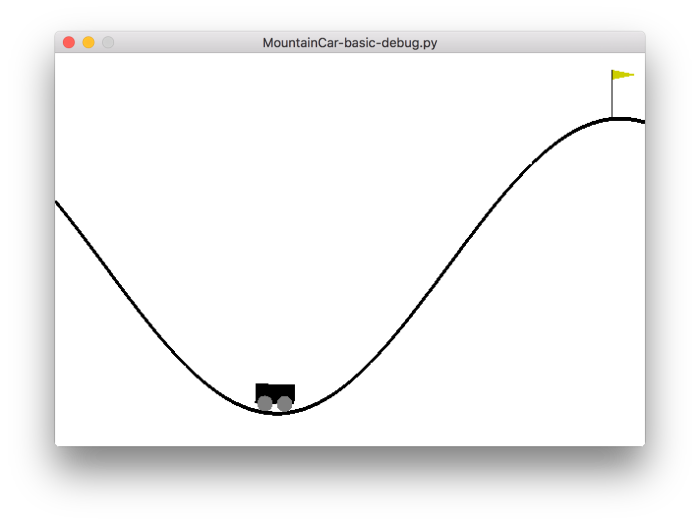
The game is simple classic control, where the car swings back and forth until it gathers enough momentum to reach the top of the hill where the flag is. The car is observed based on its position state with these values and assignments:
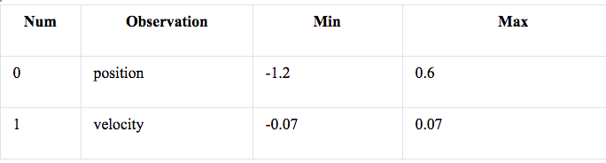
Three actions can be made upon these observations. The car can push left (action 0), push right (action 2), or not push at all (action 1). The goal of is to make the right string of actions to swing the car up the hill. For each given action taken, a reward is assigned to the action at that state. The reward is given as -1 for each time step. And the reward continues to decrease by that negative step until the position reaches a value of 0.5 from its starting value -- which is a stationary state with a random value between -0.6 and -0.4. If the goal is not reached, the episode ends once 200 time step iterations have been undergone.
Q-Learning
For a given state s, a decision can be made based on any available state a. At the next time step, a new state s’ is randomly chosen -- with a corresponding reward R(s, s’) following. The action a in state s determines whether the decision process will move to sI independently of the previous states. In other words, the transition process, Pa(s, s’), relies only on the previous state and action. (https://en.wikipedia.org/wiki/Markov_decision_process)
Put simply, Q-Learning finds the expected utility of a Markov decision by finding the optimal policy -- which, once a decision has been learned, can be the highest-value action. For each state, a reward is given (as would be expected for a Markov model), and, thus, the agent can maximize the future (and total) reward by picking states based on their reward. The reward is calculated as “a weighted sum of the expected values of the rewards of all future steps starting from the current state, where the weight for a step from a state Δt steps into the future is calculated as 𝛾Δt ” (https://en.wikipedia.org/wiki/Q-learning#Implementation). In this case, gamma is the “likelihood to succeed” at each step -- a number between 0 and 1 that balances rewards between steps, optimizing long-term reward, known as a discount factor. A higher discount factor will mean that rewards will propagate further back, including more states. (https://cs.stackexchange.com/questions/44905/the-meaning-of-discount-factor-on-reinforcement-learning)
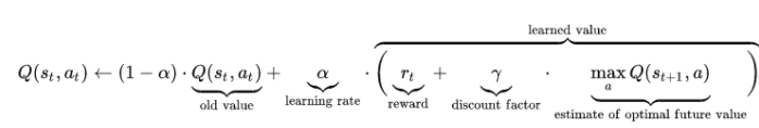
In this algorithm, the alpha represents the learning rate, which indicates the extent to which previous steps are included in calculation. An alpha of 1 would force the algorithm to include recent state values -- this value would be used in non-random, aka fully deterministic, models. Conversely, for a fully random (stochastic) model, an alpha of 0 would be used so that no previous information is used: the 0 in this algorithm would make the reward and discount factor obsolete and multiply the old Q value by a factor of 1. Thus, the old value remains the same for Q when the learning rate is 0.
When applying Q-learning to programming, the process is often slowed by the large number of states. Therefore, neural networks or function approximator algorithms are paired with Q-learning in order to increase speed by accounting for unseen states. This method can also be applied to MDP’s with finite steps through the same process.
Mountain Car is a Markov Decision Process -- it has a finite set of actions a (3) at each state. Q-learning is a suitable model to “solve” (reach the desired state) because it’s goal is to find the expected utility (score) of a given MDP. To solve Mountain Car that’s exactly what you need, the right action-value pairs based on the rewards given.
Implementation
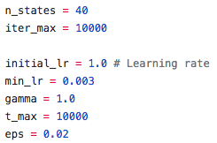
I found the original source code from malzantot on Github. He implemented a Q-learning system that originally employed a fully deterministic model; he set the learning rate (initial_lr) and the discount factor (gamma) both to 1.0. Later, he decreases the learning rate at each time step, so he also sets a minimum learning rate (min_lr) to 0.03 -- thus, letting the program never become fully stochastic. In addition, he set the number of action-value states (n_states) to 40, the epsilon random comparison value (eps) to 0.02, the max number of action-value checks per episode to 10000 (t_max), and the total number of episodes that the program will run to 10000 (iter_max).
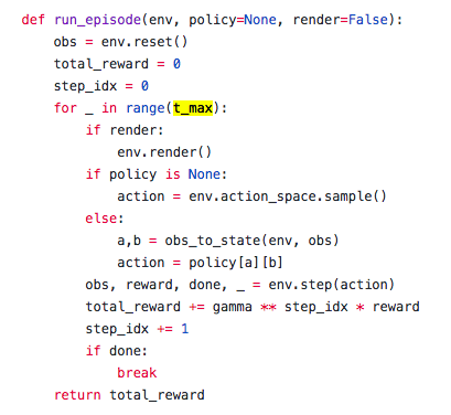
He then created a function to run the episode, letting the policy start null. This function sets the observation based on the environment and then runs observation assignment through a loop that ends at t_max. Within the loop, there are two paths: if there is no policy, assign the action to be a random based off the observation, or if a policy exists, let the action equal that policy. Observation, action, and reward are defined by the environment’s state. Then, the function returns the total reward, which increases at each step of the loop by the discount factor to the power of the current step of the loop multiplied by the reward. To end the function, the step is increased and the total reward is returned.
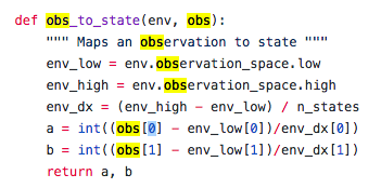
He then maps the observation to the state by finding the change between the highest and lowest possible observations (position: 0.6 and velocity: 0.07 | position: -1.2 and velocity: -0.07). Taking the difference between these high to low observations divided by the number of states, that difference minus the the first two observations, respectively, will be assigned to “a” and b,” which are used to choose a policy and location in the q table later.
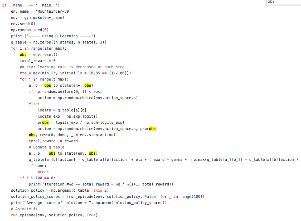
Then, the action is chosen and the average reward. He starts by creating the environment and then seeding it so that the program can be rerun and get the same values again. The q table is then created, an array initialized with 0’s (numpy.zeros). The episodes are run for a maximum number of iterations (iter_max). To start, he initializes the total reward to 0, and then decreases the learning rate at each time step to give less large and sporadic results; as it continues to iterate, it doesn’t go back to the same state each time. He initializes the q table values to the observed positions from the environment (a,b = obs_to_state (env, obs)), and then allows the program to explore new states by creating a random epsilon comparison (eps). If the random choice is not less than epsilon, he finds the exponential of all of the q table values (logits_exp), divides that by the sum of all of the table values (probs), and then assigns an action based on the environment and that value. The total reward is increased. Finally, the q learning in the given iteration occurs -- this line is simply the equation in the Q-learning section. After all of the iterations have elapsed, the average policy is found by running run_episode based on the policy found by the q table. Finally, the environment is run.
Results
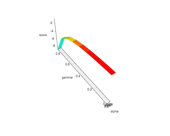
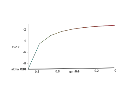
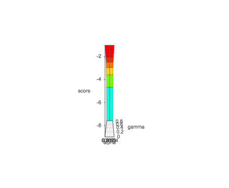
With his fully deterministic model, the result was an average score of -132.57. I then experimented with changing the alphas, beginning with making the alpha fully stochastic. In doing so, the program did not solve the environment, yielding a score of -200. In further preliminary testing, I realized that from an alpha of 0-0.625, with the random alphas I chose, the environment was solved only once. Beyond 0.625, the solution was solved, in 2 cases above .9, faster than a fully deterministic model. Thus, to experiment with alpha-gamma pairs. I set alpha to start through the loop starting at 0.8 and let gamma start at 0 and go up to 1 by increments of 0.1. The result was below. On an X-Y scale 2-D dimension, it appears to be logarithmic, and the values of score increase as the alpha-gamma value increases. This stopped before the alpha could reach 0.9 due to issues with running. However, from preliminary testing, the best alpha-gamma value was reached above 0.9, and 1, respectively.