The goal of the pendulum-v0 problem is to swing a frictionless pendulum upright so it stays vertical, pointed upwards. The pendulum starts in a random position every time, and, since pendulum-v0 is an unsolved environment, it does not have a specified reward threshold at which it is considered solved nor at which the episode will terminate.

There are three observation inputs for this environment, representing the angle of the pendulum (0 and 1) and its angular velocity (2).

The action is a value between -2.0 and 2.0, representing the amount of left or right force on the pendulum.

The precise equation for reward is: -theta2 + 0.1*theta_dt2 +0.001*action2.

Theta is normalized between -pi and pi. Therefore, the lowest cost is -(π2 + 0.1*82 + 0.001*22) = -16.2736044, and the highest cost is 0. In essence, the goal is to remain at zero angle (vertical), with the least rotational velocity, and the least effort.

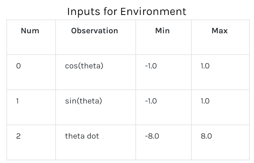
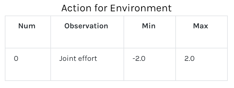
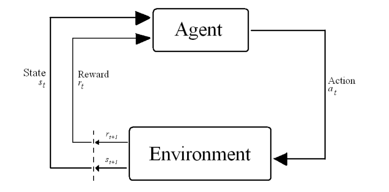
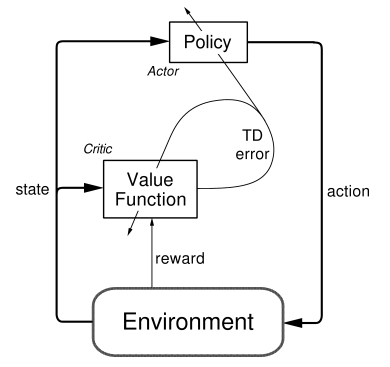
The agent learns by acting in the environment. Tasks in Reinforcement Learning are often modeled as Markov Decision Processes in which optimal actions over the state space S have to be found to optimize the total return over the process. At timestep t the agent is in state s and takes an action a ε A(s), where A(s) is the set of possible actions in s. It then transitions to state s_t+1 and receives a reward r _t+1 ε ℜ. ¹

This process is outlined here:

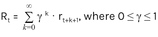
Based on this interaction the agent must learn the optimal policy π^*: S --> A to optimize the total return for a continuous task. ²

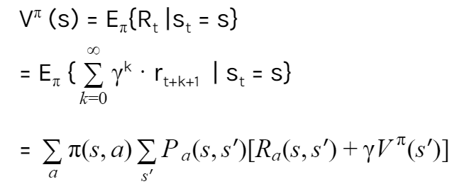
In Reinforcement Learning, learning the optimal policy is based on estimating state-value function, which expresses the value of being in a certain state. When the model of the environment is known, one can predict to what state each action will lead, and choose the action that leads to the state with the highest value.

The value for a certain state following policy π is given by this complicated Bellman Equation where π(s, a) is the chance of taking action a in s. ³

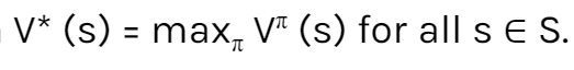
Therefore, the agent can learn the optimal policy π^* by learning the optimal state-value function: . ⁴

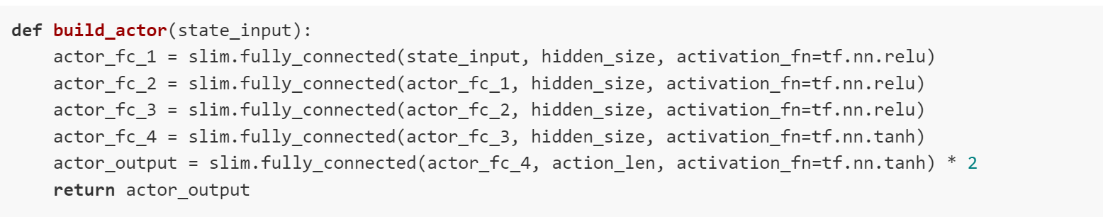
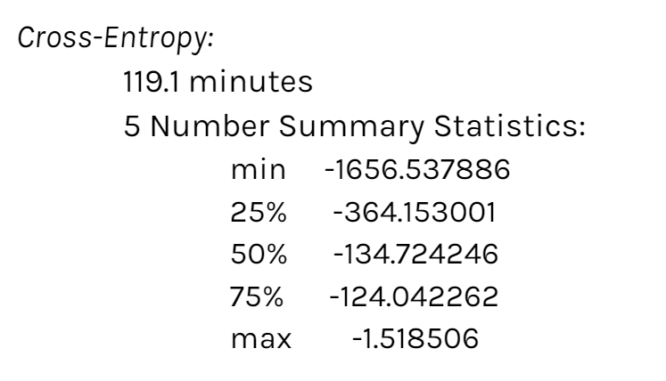
The task for the Cross Entropy method is to optimize the weights of this state-value function V(s), which determines the action of the agent, for each state using a linear value function with weights w and features Φ defining the value of a state for n features.

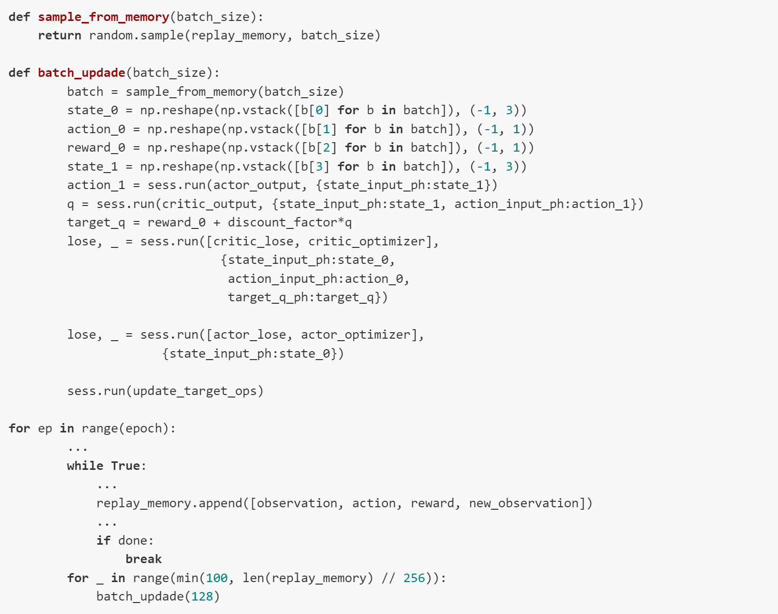
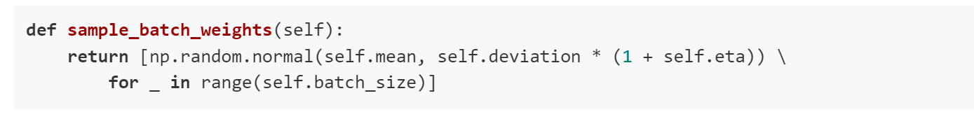
The core idea of the CE method is to sample the problem space and approximate the distribution of good solutions by assuming a distribution of the problem space, sampling the problem domain by generating candidate solutions using the distribution, and updating the distribution based on the better candidate solutions discovered. Samples are constructed step-wise (one component at a time) based on the summarized distribution of good solutions. As the algorithm progresses, the distribution becomes more refined until it focuses on the area or scope of optimal solutions in the domain. ⁵

The random sample is generated here:


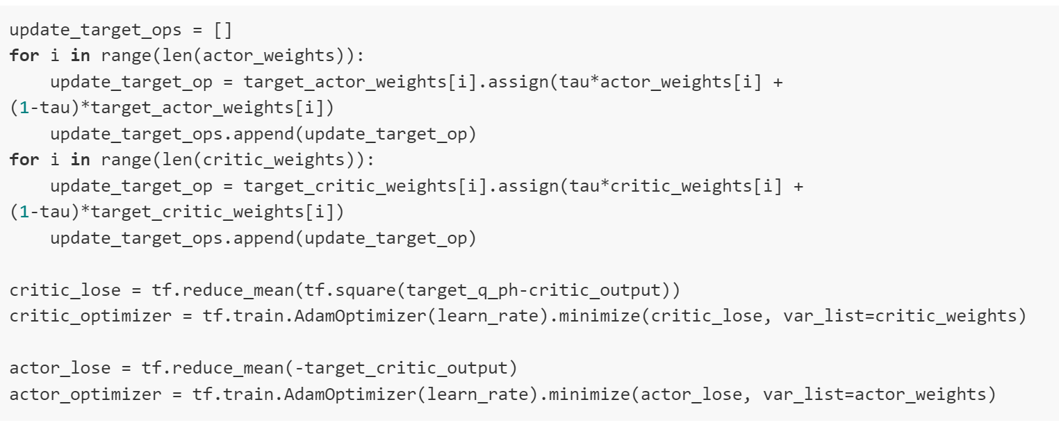
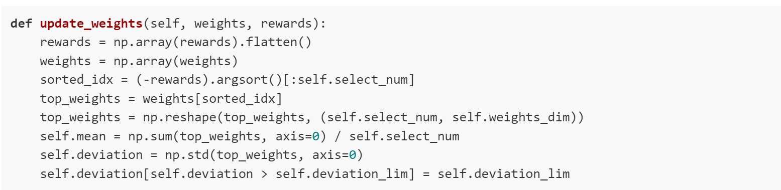
Weights are updated here to produce a better sample in the next iteration:

---

<sup>1. ["Cross Entropy Method for Reinforcement Learning" by Steijn Kistemaker http://citeseerx.ist.psu.edu/viewdoc/download?doi=10.1.1.224.3184&rep=rep1&type=pdf]↩
2. [ibid]↩
3. [ibid]↩
4. [ibid]↩
5. [ibid]↩</sup>

Policy-Gradient (PG) algorithms optimize a policy end-to-end by computing noisy estimates of the gradient of the expected reward of the policy and then updating the policy in the gradient direction. ⁶

"The Actor-Critic learning algorithm is used to represent the policy function independently of the value function. The policy function structure is known as the actor, and the value function structure is referred to as the critic."⁷

These actor and critic networks compute the action for the current state and generate a temporal-difference (TD) error signal each time step.

The input of the actor network is the current state, and the output is a value representing an action chosen from a continuous action space. The deterministic policy gradient theorem provides the update rule for the weights of the actor network. ⁸


The critic’s input is the current state and the action given by the actor, and its output is the estimated Q-value. The critic network is updated from the gradients obtained from the TD error signal. The output of the critic drives learning in both the actor and the critic. ⁹


In general, training and evaluating the policy and/or value function with thousands of temporally-correlated simulated trajectories leads to the introduction of enormous amounts of variance in the critic’s approximation of the Q-function. The TD error signal is excellent at compounding the variance introduced by your bad predictions over time. Therefore, a replay buffer is used to store the experiences of the agent during training, and then randomly sample experiences to use for learning in order to break up the temporal correlations within different training episodes. This technique is known as experience replay: ¹⁰


The last critical component is the implementation of target networks. "Directly updating your actor and critic neural network weights with the gradients obtained from the TD error signal that was computed from both your replay buffer and the output of the actor and critic networks causes your learning algorithm to diverge (or to not learn at all)." ¹¹ Therefore using a set of target networks to generate targets for TD error computation, constraining the targets to train slowly, regularizes the learning algorithm and increases stability. ¹²

---

<sup>6. ["Deep Deterministic Policy Gradients in Tensorflow" by Patrick Emami http://pemami4911.github.io/blog/2016/08/21/ddpg-rl.html ]↩
7. [ibid]↩
8. [ibid]↩
9. [ibid]↩
10. [ibid]↩
11. [ibid]↩
12. ["Continuous Control with Deep Reinforcement Learning" by Lillicrap et. al. https://arxiv.org/pdf/1509.02971.pdf]↩</sup>

The Cross-Entropy Method must learn to swing up and stay balanced, which explains its significantly longer run time (119.1 minutes compared to DDPG’s 30.3). The Actor-Critic algorithm rapid learning process is evident through its difference in rewards from epoch 0 to about epoch 20. These two phenomena explain the difference in these two distributions’ spreads: the CE Method’s IQR was 239.11 while the DDPG Method’s IQR was 73.06. However, in the end, the two methods median scores were almost identical: the median reward was -134.72 for the CE Method and -133.21 for the DDPG Method.

It would be interesting to see if these trends also apply to other OpenAI environments or if this relationship is environment specific. Additionally, it would be intriguing to examine the effect of varying these methods’ hyperparameters on their performance over time.